Lens Tutorial
We have prepared a Lens tutorial in the form of a Jupyter notebook. A static
version is reproduced below, but you can also execute it yourself by downloading
the notebook file.
Lens Tutorial
Lens is a library for exploring data in Pandas DataFrames. It computes single column summary statistics and estimates the correlation between columns.
We wrote Lens when we realised that the initial steps of acquiring a new dataset were almost formulaic: what data type is in this column? How many null values are there? Which columns are correlated? What's the distribution of this value? Lens calculates all this for you, and provides convenient visualisation of this information.
You can use Lens to analyse new datasets as well as using it to compare how DataFrames change over time.
Using lens
To start using Lens you need to import the library:
import lens
Lens has two key functions; lens.summarise for generating a Lens Summary from a DataFrame and
lens.explore for visualising the results of a summary.
For this tutorial we are going to use Lens to analyse the Room Occupancy dataset provided in the Machine Learning Repository of UC Irvine. It includes ambient information about a room such as Temperature, Humidity, Light, CO2 and whether it was occupied. The goal is to predict occupancy based on the room measurements.
We read the training portion of the dataset into pandas directly from the UCI repository:
import pandas as pd
from urllib.request import urlopen
from io import BytesIO
from zipfile import ZipFile

remote_zip = urlopen('https://archive.ics.uci.edu/ml/machine-learning-databases/00357/occupancy_data.zip')
df = pd.read_csv(BytesIO(ZipFile(BytesIO(remote_zip.read())).read('datatraining.txt')))

# Split a numerical variable to have additional categorical variables
df['Humidity_cat'] = pd.cut(df['Humidity'], 5,
                            labels=['low', 'medium-low', 'medium',
                                    'medium-high', 'high']).astype('str')
print('Number of rows in dataset: {}'.format(len(df.index)))
df.head()
Creating the summary
When you have a DataFrame that you'd like to analyse the first thing to do is
to create a Lens Summary object.
ls = lens.summarise(df)
The summarise function takes a DataFrame and returns a Lens Summary object. The
time this takes to run is dependent on both the number of rows and the number of
columns in the DataFrame. It will use all cores available on the machine, so you
might want to use a SherlockML instance with more cores to speed up the computation
of the summary. There are additional optional parameters that can be
passed in. Details of these can be found in the summarise API docs.
Given that creating the summary is computationally intensive, Lens provides a way to save this summary to a JSON file on disk and recover a saved summary through the to_json and from_json methods of lens.summary. This allows to store it for future analysis or to share it with collaborators:
# Saving to JSON
ls.to_json('room_occupancy_lens_summary.json')

# Reading from a file
ls_from_json = lens.Summary.from_json('room_occupancy_lens_summary.json')
The LensSummary object contains the information computed from the dataset and provides methods to access both column-wise and whole dataset information. It is designed to be used programatically, and information about the methods can be accessed in the LensSummary API docs.
print(ls.columns)
Create explorer
Lens provides a function that converts a Lens Summary into an Explorer object.
This can be used to see the summary information in tabular form and to display
plots.
explorer = lens.explore(ls)
Coming back to our room occupancy dataset, the first thing that we'd like to know is a high-level overview of the data.
Describe
To show a general description of the DataFrame call the describe function.
This is similar to Pandas' DataFrame.describe but also shows information for non-numeric columns.
explorer.describe()
We can see that our dataset has 8143 rows and all the rows are complete. This
is a very clean dataset! It also tells us the columns and their types, including a desc field that explains how Lens will treat this column.
Column details
To see type-specific column details, use the column_details method. Used on a numeric column such as Temperature, it provides summary statistics for the data in that column, including minimun, maximum, mean, median, and standard deviation.
explorer.column_details('Temperature')
We saw in the ouput of explorer.describe() that Occupancy, our target variable, is a categorical column with two unique values. With explorer.column_details we can obtain a frequency table for these two categories - empty (0) or occupied (1):
explorer.column_details('Occupancy')
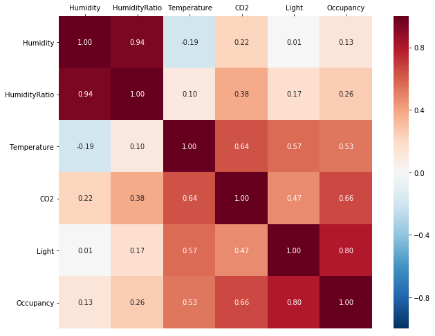
Correlation
As a first step in exploring the relationships between the columns we can look at the correlation coefficients. explorer.correlation() returns a Spearman rank-order correlation coefficient matrix in tabular form.
explorer.correlation()
However, parsing a correlation table becomes difficult when there are many columns in the dataset. To get a better overview, we can plot the correlation matrix as a heatmap, which immediately highlights a group of columns correlated with Occupancy: Temperature, Light, and CO2.
explorer.correlation_plot()
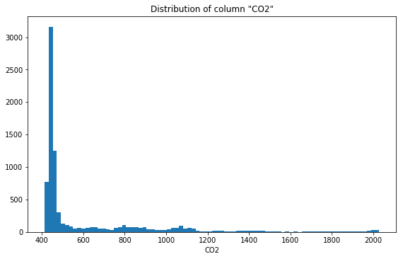
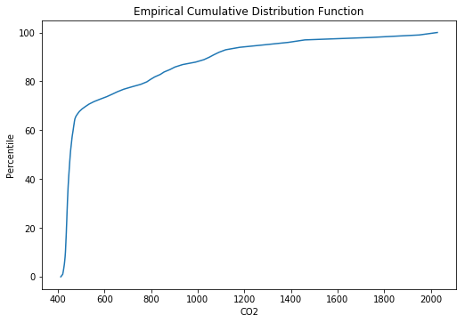
Distribution and Cumulative Distribution
We can explore the distribution of numerical variables through the distribution_plot and cdf_plot functions:
explorer.distribution_plot('Temperature')
explorer.cdf_plot('Temperature')
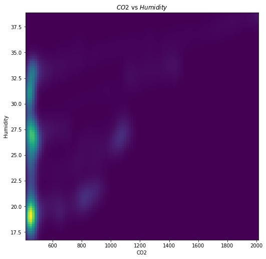
Pairwise plot
Once we know that certain columns might be correlated, it is useful to visually explore that correlation. This would typically be done through a scatter plot, and Lens has computed a 2D Kernel Density Estimate of the scatter plot that can be accessed through pairwise_density_plot.
explorer.pairwise_density_plot('Temperature', 'Humidity')
pairwise_density_plot can also show the relationship between a numeric column and a categorical column. In this case, a 1D KDE is computed for each of the categories in the categorical column.
explorer.pairwise_density_plot('Temperature', 'Occupancy')
Crosstab
The pairwise relationship between two categorical variables can also be seen as a cross-tabulation: how many observations exist in the dataset of the combination of categories in the two variables. This can be seen as a table or as a plot, which can be useful when the number of categories is very large.
explorer.crosstab('Occupancy', 'Humidity_cat')
explorer.pairwise_density_plot('Occupancy', 'Humidity_cat')
Interactive widget
An alternative way of quickly exploring the plots available in Lens is through a Jupyter widget provided by lens.interactive_explore. Creating it is as easy as running this function on a Lens Summary.
Note that if you are reading this tutorial through the online docs the output of the following cell will not be interactive as it needs to run within a notebook. Download the notebook from the links below to try out the interactive explorer!
lens.interactive_explore(ls)

(room_occupancy_example.ipynb; room_occupancy_example_evaluated.ipynb; room_occupancy_example.py)